Visualization of near field

MSTM code can be used to calculate the distribution of the near (or local) field. The field is calculated on a rectangular region, specified by input (nearfield.NearField.set_plane()). Currently, only magnititude of electric field \(|E|^2\) can be visualized.

Example: field distribution near two particles

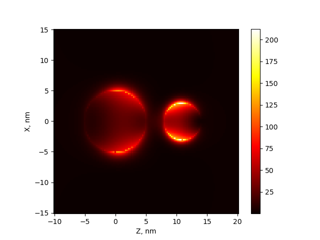
Two silver spheres with radii 5 and 3 nm are placed at 0,0,0 and 0,0,11. Incident beam with wavelength 385 nm is directed by Z axis and have X polzarization.

from mstm_studio.nearfield import NearField
from mstm_studio.mstm_spectrum import ExplicitSpheres
from mstm_studio.alloy_AuAg import AlloyAuAg

mat = AlloyAuAg(x_Au=0.0)       # silver material
nf = NearField(wavelength=385)  # near the resonance
nf.environment_material = 1.5   # glass matrix
nf.set_plane(plane='xz', hmin=-10, hmax=20, vmin=-15, vmax=15, step=0.25)

spheres = ExplicitSpheres(2, [0, 0, 0, 5, 0, 0, 11, 3],
                          mat_filename=2*[mat])
nf.set_spheres(spheres)

nf.simulate()

nf.plot()

Resulting image

Class

class mstm_studio.nearfield.NearField(wavelength)

Calculate field distribution map at fixed wavelength

plot(fig=None, axs=None, caxs=None)

Show 2D field distribution

Parameters:

fig:

matplotlib figure

axs:

matplotlib axes

caxs:

matplotlib axes for colorbar

Returns:

filled/created fig and axs objects

set_plane(plane='zx', hmin=-10.0, hmax=10.0, vmin=-10.0, vmax=10.0, step=1.0, offset=0.0)

Determine the plane and grid for near field computation.

plane: one of ‘yz’|’zx’|’xy’ hmin, hmax, vmin, vmax: horizontal and vertical sizes step: size of the grid grain offset: shift of the plane

simulate()

Run MSTM code to produce 2D map of field distribution.

write(filename)

save field data to text file