Materials
The materials are characterized by refractive index, which is a square root (complex valued) of macroscopic dielectric function. Generally, this should be the spectral function, i. e.
so that
with \(\hbar \omega = 2 \pi \hbar c / \lambda\).
Constant Material
The material with constant refreactive index can be specified as first constructor argument (file_name):
>>> from mstm_studio.mstm_spectrum import Material
>>> mat_glass = Material('1.5')
>>> mat_glass.get_n(500)
array(1.5)
Complex value can be supplied too:
>>> mat_lossy = Material('3+1j')
>>> mat_lossy.get_n(500)
array(3.)
>>> mat_lossy.get_k(500)
array(1.)
Also the predifned names can be used: air, water, glass.
Loading from file
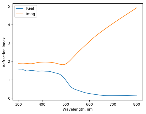
The tabular data on refractive index is convinient to store in file.
The header of the file required to have special labels: lambda n k. The example file “etaGold.txt” can be found in directory “nk” of source distribution.
Assuming the file “etaGold.txt” is in the same directory where script is running, it can be loaded with
gold = Material('etaGold.txt')
fig, axs = gold.plot()
fig.savefig('loaded_gold.png', bbox_inches='tight')
Resulted plot
Note
The extending database of refractive indeces of materials <https://refractiveindex.info/>.
Material from numpy array
Material data can be specified directly by numpy (complex) array by passing nk or eps. Next examples shows loading of Drude-like dielectric function:
from mstm_studio.mstm_spectrum import Material
import numpy as np

wls = np.linspace(300, 800, 51)  # spectral region
omega = 1240. / wls              # freq. domian

omega_p = 9.        # plasma frequency, eV
gamma   = 0.03      # damping, eV
# Drude's dielectric function:
epsilon = 1 + omega_p**2 / (omega * (omega - 1j * gamma))

mat = Material('drude', eps=epsilon, wls=wls)
Material class members
- class mstm_studio.mstm_spectrum.Material(file_name, wls=None, nk=None, eps=None)[source]
Material class.
Use get_n() and get_k() methods to obtain values of refraction index at arbitraty wavelength (in nm).
Parameters:
- file_name:
complex value, written in numpy format or as string;
one of the predefined strings (air, water, glass);
filename with optical constants.
File header should state lambda, n and k columns If either nk= n + 1j*k or eps = re + 1j*im arrays are specified, then the data from one of them will be used and filename content will be ignored.
- wls: float array
array of wavelengths (in nm) used for data interpolation. If None then
np.linspace(300, 800, 500)will be used.
Analytical formula for AuAg
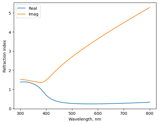
Silver, gold and thier alloy materials can be specified using analytical expression proposed in the study [Rioux2014]. Example for Au:Ag = 1:2 alloy:
from mstm_studio.alloy_AuAg import AlloyAuAg

au1ag2 = AlloyAuAg(x_Au=1./3)
fig, axs = au1ag2.plot()
fig.savefig('mat_au1ag2.png', bbox_inches='tight')
Resulted plot
- class mstm_studio.alloy_AuAg.AlloyAuAg(x_Au)[source]
Material class for AuAg alloys.
Use get_n() and get_k() to obtain values of refraction indexes (real and imaginary) at arbitraty wavelength (in nm) by model and code from Rioux et al doi:10.1002/adom.201300457
Parameters:
- x_Au: float
fraction of gold
Materials from RefractionIndex.Info
Online database of materials RII [RII] <https:\refractiveindex.info> provides dielectric functions of a several hundreds of materials. Up to Dec 2024 it contains 445 different materials (“books” in RII notation) and 163 of them are suitable for calculations in MSTM-Studio (i.e. contain tabulated data with wavelength in interval from 300 to 800 nm).
Materials can be loaded from the local dump of online database, which can be obtained from the official RII website (About->Resources, direct link: <https://refractiveindex.info/download/database/rii-database-2024-12-31.zip>).
By default mstm_studio will search for rii-database-*.zip archive in home directory and in application data directory. The exact location may be determined in argument of class constructor.
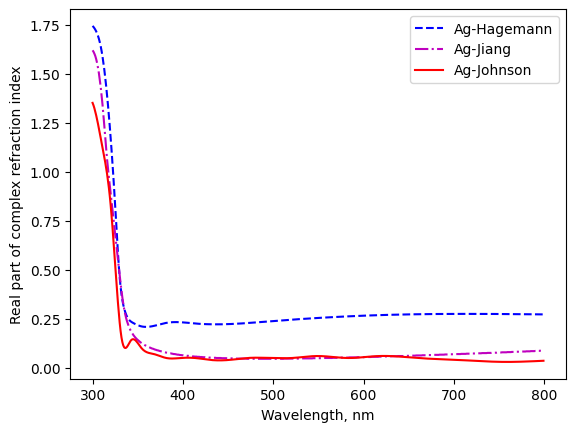
Example: Compare refraction indeces of silver of different authors
import numpy as np
import matplotlib.pyplot as plt
from mstm_studio.rii_materials import RiiMaterial

wls = np.arange(300, 800, 1)

mat = RiiMaterial()  # search RII archive in default paths
mat.scan()           # fill db items
print(mat.rii_db_items['main']['Ag'])
# ['Babar', 'Choi', 'Ciesielski', 'Ciesielski-Ge', 'Ciesielski-Ni',
#  'Ferrera-298K', 'Ferrera-404K', 'Ferrera-501K', 'Ferrera-600K',
#  'Hagemann', 'Jiang', 'Johnson', 'McPeak', 'Rakic-BB', 'Rakic-LD',
#  'Stahrenberg', 'Werner', 'Werner-DFT', 'Windt', 'Wu', 'Yang']

mat.select('main', 'Ag', 'Hagemann')
plt.plot(wls, mat.get_n(wls), 'b--', label='Ag-Hagemann')

mat.select('main', 'Ag', 'Jiang')
plt.plot(wls, mat.get_n(wls), 'm-.', label='Ag-Jiang')

mat.select('main', 'Ag', 'Johnson')
plt.plot(wls, mat.get_n(wls), 'r-', label='Ag-Johnson')


plt.legend()
plt.xlabel('Wavelength, nm')
plt.ylabel('Real part of complex refraction index')
Resulted plot
- class mstm_studio.rii_materials.RiiMaterial(archive_filename='')[source]
Setup material from RefractiveIndexInfo database dump available online at url: <https://refractiveindex.info/download/database/>
- archive_filename: string
path to the downloaded zip file of db dump
Example of usage: >>> riimat = RiiMaterial(‘rii-database-2024-08-14.zip’) >>> riimat.select(‘main’, ‘Ag’, ‘Babar’)
- count_materials()[source]
Return the number of distinct materials (not including variants of dielectric functions)
- filter_valid()[source]
Remove materials from the internal dict rii_db_items which does not contain data in limit of 300 and 800 nm
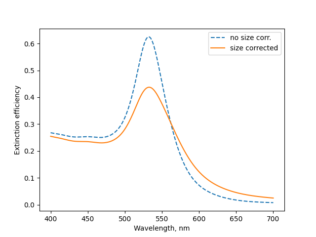
Size correction for dielectric functions
Macroscopic dielectric function obtained for bulk samples can be applied to nanoparticles with caution. It is claimed that only particles of radius above 10 nm can be considered. However, the consideration can be extended to the sizes down to ~ 2 nm by inclusion of the most prominent effect – the decrease of the mean free path length of electrons due to finite size of the nanoparticles. The correction is applied to the \(\gamma\) parameter of the Drude function, so that we had to add the contribution
to the experimental dielectric function given by the table.
Example for 3 nm gold nanoparticle:
from mstm_studio.mstm_spectrum import Material
from mstm_studio.diel_size_correction import SizeCorrectedGold
from mstm_studio.contributions import MieSingleSphere
import numpy as np
import matplotlib.pyplot as plt

D = 3  # particle size
wls = np.linspace(400, 700, 201)  # spectral region

gold = Material('etaGold.txt')  # bulk dielectric function
gold_corr = SizeCorrectedGold('etaGold.txt')  # corrected, D-dependent

mie = MieSingleSphere(wavelengths=wls, name='MieSphere')

mie.set_material(material=gold, matrix=1.5)
plt.plot(wls, mie.calculate(values=[1, D]), '--', label='no size corr.')

mie.set_material(material=gold_corr, matrix=1.5)
plt.plot(wls, mie.calculate(values=[1, D]), label='size corrected')
Resulted plot
Currently the corrections for gold and silver are implemented:
- class mstm_studio.diel_size_correction.SizeCorrectedGold(file_name, wls=None, nk=None, eps=None)[source]
Size correction for gold dielectric function (mean free path is limited by particle size) according to
A. Derkachova, K. Kolwas, I. Demchenko Plasmonics, 2016, 11, 941 doi: <10.1007/s11468-015-0128-7>
- class mstm_studio.diel_size_correction.SizeCorrectedSilver(file_name, wls=None, nk=None, eps=None)[source]
Size correction for gold dielectric function (mean free path is limited by particle size) according to
J.M.J. Santillán, F.A. Videla, M.B.F. van Raap, D. Muraca, L.B. Scaffardi, D.C. Schinca J. Phys. D: Appl. Phys., 2013, 46, 435301 doi: <10.1088/0022-3727/46/43/435301>
Also the general correction class is available:
- class mstm_studio.diel_size_correction.SizeCorrectedMaterial(file_name, wls=None, nk=None, eps=None, omega_p=10.0, gamma_b=0.1, v_Fermi=1.0, sc_C=0.0)[source]
Create material with correction to the finite crystal size. Only life-time limit (~1/gamma) is considered. This should be sufficient for the sizes above ~2 nm. The particles smaller than ~2 nm require more sofisticated modifications (band gap, etc.)
Parameters:
- file_name, wls, nk, eps:
same meanining as for Material
Parameters for size correction:
- omega_p:
plasma frequency (bulk) [eV]
- gamma_b:
life-time broadening (bulk) [eV]
- v_Fermi:
Fermi velocity (bulk) [nm/fs]
- sc_C:
size-corr. adj. parameter [unitless]
size of the particle is specified as self.D
Rioux, S. Vallières, S. Besner, P. Muñoz, E. Mazur, and M. Meunier, “An Analytic Model for the Dielectric Function of Au, Ag, and their Alloys” Adv. Opt. Mater. (2014) 2 176-182 <http://dx.doi.org/10.1002/adom.201300457>
Polyanskiy, “Refractiveindex.info database of optical constants” Sci. Data (2024) 11, 94 <https://doi.org/10.1038/s41597-023-02898-2>