Simple functions and Mie theory
Example
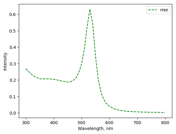
The example how to obtain contribution to the extinction from Log-Normally distributed spheres. Other contributions are evaluated in similar way.
from mstm_studio.contributions import MieLognormSpheres
from mstm_studio.alloy_AuAg import AlloyAuAg
import numpy as np
mie = MieLognormSpheres(name='mie', wavelengths=np.linspace(300,800,51))
mie.set_material(AlloyAuAg(x_Au=1), 1.5) # golden sphere in glass
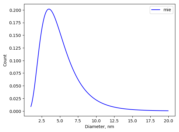
values = [1, 1.5, 0.5] # scale, mu, sigma
fig, _ = mie.plot(values)
fig.savefig('mie_contrib.png', bbox_inches='tight')
mie.MAX_DIAMETER_TO_PLOT = 20   # 100 nm is by default
fig, _ = mie.plot_distrib(values)
fig.savefig('mie_distrib.png', bbox_inches='tight')
Classes
Contributions to UV/vis extinction spectra other then obtained from MSTM.
- class mstm_studio.contributions.ConstantBackground(wavelengths=[], name='ExtraContrib')[source]
Constant background contribution \(f(\lambda) = bkg\).
Parameters:
- wavelengths: list or numpy array
wavelengths in nm
- name: string
optional label
- class mstm_studio.contributions.Contribution(wavelengths=[], name='ExtraContrib')[source]
Abstract class to include contributions other then calculated by MSTM. All lightweight calculated contribtions (constant background, lorentz and guass peaks, Mie, etc.) should enhirit from it.
Parameters:
- wavelengths: list or numpy array
wavelengths in nm
- name: string
optional label
- calculate(values)[source]
This method should be overriden in child classes.
Parameters:
values: list of control parameters
Return:
numpy array of contribution values at specified wavelengths
- class mstm_studio.contributions.GaussPeak(wavelengths=[], name='ExtraContrib')[source]
Gauss function
\[G(\lambda) = scale \cdot \exp\left( - \frac{(\lambda-\mu)^2}{2\sigma^2} \right)\]Parameters:
- wavelengths: list or numpy array
wavelengths in nm
- name: string
optional label
- class mstm_studio.contributions.LinearBackground(wavelengths=[], name='ExtraContrib')[source]
Two-parameter background \(f(\lambda) = a \cdot \lambda + b\).
Parameters:
- wavelengths: list or numpy array
wavelengths in nm
- name: string
optional label
- class mstm_studio.contributions.LorentzBackground(wavelengths=[], name='ExtraContrib')[source]
Lorentz peak in background. Peak center is fixed.
\[L(\lambda) = \frac {scale} {(\lambda-center)^2 + \Gamma^2}\]Parameters:
- wavelengths: list or numpy array
wavelengths in nm
- name: string
optional label
- class mstm_studio.contributions.LorentzPeak(wavelengths=[], name='ExtraContrib')[source]
Lorentz function
\[L(\lambda) = \frac {scale} {(\lambda-\mu)^2 + \Gamma^2}\]Parameters:
- wavelengths: list or numpy array
wavelengths in nm
- name: string
optional label
- class mstm_studio.contributions.MieLognormSpheres(wavelengths=[], name='ExtraContrib')[source]
Mie contribution from an ensemble of spheres with sizes distributed by Log-Normal law
Parameters:
- wavelengths: list or numpy array
wavelengths in nm
- name: string
optional label
- calculate(values)[source]
Parameters:
values: list of control parameters scale, mu and sigma
Return:
Mie extinction efficiency of log-normally distributed spheres
- lognorm(x, mu, sigma)[source]
The shape of Log-Normal distribution:
\[LN(D) = \frac {1}{D \sigma \sqrt{2\pi}} \exp\left( - \frac{(\log(D)-\mu)^2}{2\sigma^2} \right)\]
- class mstm_studio.contributions.MieLognormSpheresCached(wavelengths=[], name='ExtraContrib')[source]
Mie contribution from an ensemble of spheres with sizes distributed by Lognormal law.
Cached version - use it to speed-up fitting.
Parameters:
- wavelengths: list or numpy array
wavelengths in nm
- name: string
optional label
- class mstm_studio.contributions.MieSingleSphere(wavelengths=[], name='ExtraContrib')[source]
Mie contribution from single sphere.
Details are widely discusses, see, for example [Kreibig_book1995]
Parameters:
- wavelengths: list or numpy array
wavelengths in nm
- name: string
optional label
Kreibig, M. Vollmer, “Optical Properties of Metal Clusters” (1995) 553