Fitting¶

Fitting of experimental spectra is a powerful tool for study of plasmonic nanoparticles. Fitting with Mie theory is routinely used to provide information about particle sizes, but fitting with MSTM can solve even agglomerates (packs) of nanoparticles, where Mie theory is not applicable, see [Avakyan2017] for example. Another application is the fitting with core-shell or multi-layered particles.

The MSTM-studio used hard-coded target (penalty) function which is minimized during fitting (ChiSq):

\[\chi^2 = \sum_i \left( y_i^\text{(fit)} - y_i^\text{(dat)} \right)^2,\]

where index i enumerates wavelengths.

Example: fit with Mie theory¶

Exampels experimental file, included in distribution, is the extinction spectra of gold particles laser-impregnated in glass, synthesized and studied by Maximilian Heinz [Avakyan2017].

from mstm_studio.alloy_AuAg import AlloyAuAg
from mstm_studio.contributions import LinearBackground, MieLognormSpheresCached
from mstm_studio.fit_spheres_optic import Fitter

fitter = Fitter(exp_filename='experiment.dat')        # load experiment from tabbed file
fitter.set_extra_contributions(
    [LinearBackground(fitter.wls),                    # wavelengths from experiment
     MieLognormSpheresCached(fitter.wls, 'LN Mie')],  # cached version for faster fittting
    [0.02, 0.0001, 0.1, 2.0, 0.4])                    # initial values for a, b, C, mu, sigma
fitter.extra_contributions[1].set_material(AlloyAuAg(1.), 1.5)  # gold particles in glass
fitter.set_spheres(None)  # no spheres - no slow MSTM runs

# run fit (takes ~20 seconds on 2GHz CPU)
fitter.run()

fitter.report_result()

# plot results
import matplotlib.pyplot as plt
plt.plot(fitter.wls, fitter.exp,  'ro', label='exp.')
plt.plot(fitter.wls, fitter.calc, 'b-', label='fit')
plt.xlabel('Wavelength, nm')
plt.ylabel('Exctinction, a.u.')
plt.legend()
plt.savefig('fit_by_Mie.png', bbox_inches='tight')

Output (final part):

ChiSq:      0.000219
Optimal parameters
    ext00:  0.035177        (Varied:True)
    ext01:  -0.000049       (Varied:True)
    ext02:  0.007908        (Varied:True)
    ext03:  4.207724        (Varied:True)
    ext04:  0.284066        (Varied:True)
    scale:  7030.322097     (Varied:True)

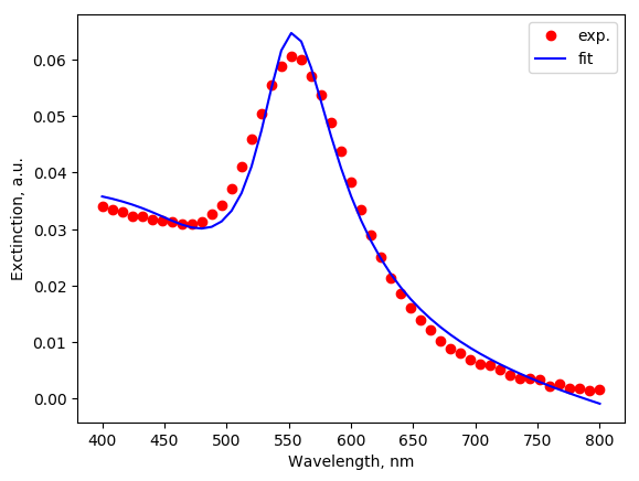
The low value of ChiSq and inspecting of agreement between theoretical and experimental curves are indicate on acceptable fitting. The names of fitting parameters are explained in Constraints subsection (see Parameter). In this example the ext00 and ext01 are the parameters a and b of linear contribution, ext02 is a scale multiplier for Mie contribution, ext03 and ext04 correspond to mu and sigma parameters of Log-Normal distribution (see mstm_spectrum.MieLognormSpheres). The last parameter, the common scale multiplier 100 % correlates with ext02, resulting in spurious absolute values. If needed, the particle concentration can be estimated from thier product \(scale \times ext02\) or by constraining one of them during fitting.

Fitter class¶

class mstm_studio.fit_spheres_optic.Fitter(exp_filename, wl_min=300, wl_max=800, wl_npoints=51, extra_contributions=None, plot_progress=False)[source]¶

Class to perform fit of experimental Exctinction spectrum

Field:

tolerance: float

stopping criterion, default is 1e-4

Parameters:

exp_filename: str

name of file with experimental data

wl_min, wl_max: float

wavelength bounds for fitting (in nm).

wl_npoints: int

number of wavelengths where spectra will be calcualted and compared.

extra_contributions: list of Contribution objects

If None, then ConstantBackground will be used. Assuming that first element is a background. If you don’t want any extra contribution, set to empty list [].

plot_progress: bool

Show fitting progress using matplotlib. Should be turned off when run on parallel cluster without gui.

add_constraint(cs)[source]¶

Adds constraints on the parameters. Usefull for the case of core-shell and layered structures.

Parameter:

cs: Contraint object or list of Contraint objects

get_extra_contributions()[source]¶: Return a list of current extra contributions to the spectrum

report_freedom()[source]¶: Returns string with short summary before fitting

report_result(msg=None)[source]¶: Returns string with short summary of fitting results

run(maxsteps=400)[source]¶

Start fitting.

Parameters:

maxsteps: int: limits number of steps performed

set_callback(func)[source]¶

Set callback function which will be called on each step of outer optimization loop.

Parameter:

func: function(values)

where values – list of values passed from optimization routine

set_extra_contributions(contributions, initial_values=None)[source]¶

Add extra contributions and initialize corresponding params.

Parameters:

contributions: list of Contribution objests

initial_values: float array

set_matrix(material='AIR')[source]¶

set refraction index of matrix material

material : {‘AIR’|’WATER’|’GLASS’} or float: the name of material or refraction index value.

set_spheres(spheres)[source]¶

Specify the spheres to be fit.

Paramerer:

spheres: list of mstm_spectrum.Sphere objects

If None then MSTM will not be run.

Constraints¶

The constraints allow to speed-up or direct the fitting. Thier setup requires specification of variable names, which are described in Parameter class documentation:

class mstm_studio.fit_spheres_optic.Parameter(name, value=1, min=None, max=None, internal_loop=False)[source]¶

Class for parameter object used for storage of parameter’s name, value and variation limits.

Parameter naming conventions:

scale - outer common multiplier

ext%i - extra parameter, like background, peaks or Mie contributions

a%i - sphere radius

x%i, y%i, z%i - coordinates of sphere center

where %i is a number (0, 1, 2, …)

Parameters:

name: string

name of parameter used for constraints etc

value: float

initial value of parameter

min, max: float

bounds for parameter variation (optional)

internal_loop : bool

if True the parameter will be allowed to vary in internal (fast) loop, which does not require MSTM recalculation. Note: this flag will be removed in future.

varied: bool

if True – will be changed during fit

Example: fit by core-shell¶

Fit the same experiment as above, but using model of core-shell particle, just to illustrate the technique.

from mstm_studio.alloy_AuAg import AlloyAuAg
from mstm_studio.contributions import LinearBackground, MieLognormSpheresCached
from mstm_studio.mstm_spectrum import ExplicitSpheres, Profiler
from mstm_studio.fit_spheres_optic import Fitter, FixConstraint, ConcentricConstraint

fitter = Fitter(exp_filename='experiment.dat')        # load experiment from tabbed file
fitter.set_extra_contributions(
    [LinearBackground(fitter.wls)],     # wavelengths from experiment
    [0.02, 0.0001])                     # initial values for a, b

spheres = ExplicitSpheres(2, [0,0,0,10,0,0,0,12], mat_filename=[AlloyAuAg(1.),AlloyAuAg(0.)])
fitter.set_spheres(spheres) # core-shell Au@Ag particle
fitter.set_matrix(1.5)      # in glass

fitter.add_constraint(ConcentricConstraint(0, 1))  # 0 -> 1
fitter.add_constraint(FixConstraint('x00'))
fitter.add_constraint(FixConstraint('y00'))
fitter.add_constraint(FixConstraint('z00'))

# run fit (takes ~200 seconds on 2GHz CPU)
with Profiler():
    fitter.run()

fitter.report_result()

# plot results
import matplotlib.pyplot as plt
plt.plot(fitter.wls, fitter.exp,  'ro', label='exp.')
plt.plot(fitter.wls, fitter.calc, 'b-', label='fit')
plt.xlabel('Wavelength, nm')
plt.ylabel('Exctinction, a.u.')
plt.legend()
plt.savefig('fit_by_core-shell.png', bbox_inches='tight')

Output (final part):

ChiSq:      0.002354
Optimal parameters
        a00:        1.284882        (Varied:True)
        a01:        1.958142        (Varied:True)
        ext00:      0.186312        (Varied:True)
        ext01:      -0.000247       (Varied:True)
        scale:      -0.063814       (Varied:True)
        x00:        0.000000        (Varied:False)
        x01:        0.000000        (Varied:False)
        y00:        0.000000        (Varied:False)
        y01:        0.000000        (Varied:False)
        z00:        0.000000        (Varied:False)
        z01:        0.000000        (Varied:False)

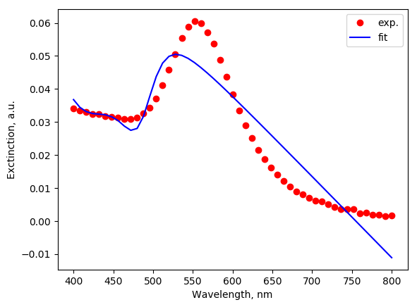
The fiting quality demonstrated by parameter ChiSq is ~10 times worse comparing when used the ensemble of non-interacting gold particles. The figure shows unacceptable fitting quality too.

Constraints classes¶

class mstm_studio.fit_spheres_optic.Constraint[source]¶

Abstract constraint class. All other should inherit from it.

apply(params)[source]¶

Modify the params dict according to given constranint algorithm.

Note: Abstract method!

class mstm_studio.fit_spheres_optic.FixConstraint(prm, value=None)[source]¶

Fix value of parameter with name prm to value.

Parameters:

prm: string

parameter name

value: float

if None than initial value will be used.

apply(params)[source]¶: Apply fix constraint

class mstm_studio.fit_spheres_optic.EqualityConstraint(prm1, prm2)[source]¶

Fix two parameters with names prm1 and prm2 being equal

apply(params)[source]¶: Apply equality constraint

class mstm_studio.fit_spheres_optic.ConcentricConstraint(i1, i2)[source]¶

Two spheres with common centers.

i1 and i2 – indexes of spheres

apply(params)[source]¶: Apply concentric constraint

class mstm_studio.fit_spheres_optic.RatioConstraint(prm1, prm2, ratio=1)[source]¶

Maintain ratio of two variables, prm1/prm2 = ratio

apply(params)[source]¶: Apply Ratio constraint

set_ratio(ratio)[source]¶: Set ratio of \(prm1/prm2 = ratio\).

[Avakyan2017]

(1, 2)

Avakyan, M. Heinz, A. Skidanenko, K. Yablunovskiy, J. Ihlemann, J. Meinertz, C. Patzig, M. Dubiel, L. Bugaev “Insight on agglomerates of gold nanoparticles in glass based on surface plasmon resonance spectrum: Study by multi-spheres T-matrix method” J. Phys.: Condens. Matter (2018) 30, 045901-045909 <https://doi.org/10.1088/1361-648X/aa9fcc>

Fitting¶

Example: fit with Mie theory¶

Fitter class¶

Constraints¶

Example: fit by core-shell¶

Constraints classes¶

MSTM-studio

Navigation

Related Topics